How to CONDUCT A EDA univariate 🗂️
Exploratory data analysis (EDA) is frequently used by data scientists or data analysts to comprehend datasets for use in decision-making and data cleansing procedures. Important facts about the data, including hidden patterns, outliers, variance, covariance, and correlations between characteristics, are revealed by EDA. The data is crucial for designing the hypothesis and building more effective models.
EDA often fits into one of two categories, univariate and multivariate analysis. Analyzing one feature, such as summarizing and identifying feature patterns, is what univariate analysis entails. The univariate exploratory data analysis works with four summary measures:
Position
Dispersion
Shape
Inequality
- Positional measures: they are the typical or representative values of the variable under study.
Arithmetic average: The arithmetic mean formula calculates the mean or average of the numbers and is used to measure the central tendency of the data. It can also be defined as the sum of all the given observations to the total number of observations.

It is the most used measure. However, it is very sensitive to outliers and extreme observations that is why, if you have outliers in our data, we should use the median.
Median: For the calculation of the median, the data has to be arranged in ascending order, and then the middlemost data point represents the median of the data. The basic feature of the median in describing data compared to the mean (often simply described as the "average") is that it is not skewed by a small proportion of extremely large or small values, and therefore provides a better representation of a "typical" value.

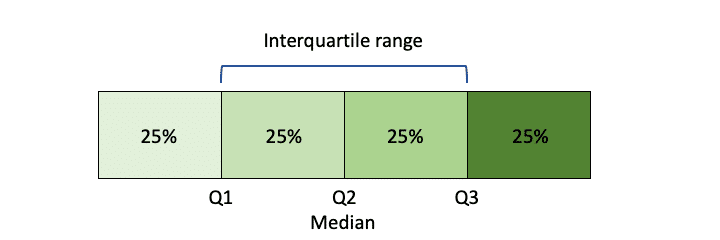
Quantile: quantiles are cut points dividing the range of a probability distribution into continuous intervals with equal probabilities, or dividing the observations in a sample in the same way. Q-quantiles are values that partition a finite set of values into q subsets of (nearly) equal sizes. There are q − 1 partitions of the q-quantiles, one for each integer k satisfying 0 < k < q.
Special cases of quantiles are quartiles when three values divide the data into four parts (Q1: leaves 25% of the observations to the left; Q2: median: leaves 50% of the observations to the left; Q3: leaves 75% of the observations to the left). Deciles: nine values that divide the data into ten parts and Percentiles when 99 values divide the data into one hundred parts

Other positional measures:
Geometric mean: the geometric mean is a mean or average, which indicates the central tendency or typical value of a set of numbers by using the product of their values (as opposed to the arithmetic mean which uses their sum). For instance, the geometric mean of two numbers, say 2 and 8, is just the square root of their product, that is,


Harmonic mean: In mathematics, the harmonic mean is one of several kinds of average, and in particular, one of the Pythagorean means. It is sometimes appropriate for situations when the average rate is desired.
The harmonic mean can be expressed as the reciprocal of the arithmetic mean of the reciprocals of the given set of observations. As a simple example, the harmonic mean of 1, 4, and 4 is

The harmonic mean is one of the three Pythagorean means. For all positive data sets containing at least one pair of nonequal values, the harmonic mean is always the least of the three means, while the arithmetic mean is always the greatest of the three and the geometric mean is always in between.
Robust means: it is a trimmed mean by 10%. I mean, it is an arithmetic mean excluding the 10% of the largest values and the 10% of the smallest values)
2. Dispersion measures: the extent to which a distribution is stretched or squeezed.
Variance: variance is the expectation of the squared deviation of a random variable from its population mean or sample mean. Variance is a measure of dispersion, meaning it is a measure of how far a set of numbers is spread out from their average value.
Standard deviation: the standard deviation is a measure of the amount of variation or dispersion of a set of values. A low standard deviation indicates that the values tend to be close to the mean (also called the expected value) of the set, while a high standard deviation indicates that the values are spread out over a wider range. A useful property of the standard deviation is that, unlike the variance, it is expressed in the same unit as the data.
Coefficient of variation: the coefficient of variation (CV), also known as relative standard deviation (RSD), is often expressed as a percentage, and is defined as the ratio of the standard deviation 


Range: In statistics, the range of a set of data is the difference between the largest and smallest values, the result of subtracting the sample maximum and minimum. It is expressed in the same units as the data.
In descriptive statistics, the range is the size of the smallest interval which contains all the data and provides an indication of statistical dispersion. Since it only depends on two of the observations, it is most useful in representing the dispersion of small data sets.
Interquartile range: In descriptive statistics, the interquartile range tells you the spread of the middle half of your distribution.
Quartiles segment any distribution that’s ordered from low to high into four equal parts. The interquartile range (IQR) contains the second and third quartiles, or the middle half of your data set. The interquartile range is an especially useful measure of variability for skewed distributions.
Semi-interquartile range: The semi-interquartile range is one-half the difference between the first and third quartiles. It is half the distance needed to cover half the scores. The semi-interquartile range is affected very little by extreme scores. This makes it a good measure of spread for skewed distributions.
3. Shape measures: Measures of shape describe the distribution (or pattern) of the data within a dataset. The distribution shape of quantitative data can be described as there is a logical order of the values, and the 'low' and 'high' end values on the x-axis of the histogram are able to be identified. they are the ones that measure the Kurtosis coefficient and Skewness. Skewness tells you the amount and direction of skew (departure from horizontal symmetry), and kurtosis tells you how tall and sharp the central peak is, relative to a standard bell curve.
Skewness: The moment coefficient of skewness of a data set is
skewness: *g*1 = *m*3 / *m*23/2
where
m*3 = ∑(*x−x̅)3 / n and
m*2 = ∑(*x−x̅)2 / n
x̅ is the mean and n is the sample size, as usual. m3 is called the **third moment of the data set. m2 is the **variance, the square of the standard deviation.
If g1 = 0, the distribution is symmetric; if g1 < 0, the distribution is negatively skewed and if g1 > 0, the distribution is positively skewed.
Kurtosis: The other common measure of shape is called kurtosis. The moment coefficient of kurtosis of a data set is computed almost the same way as the coefficient of skewness: just change the exponent 3 to 4 in the formulas:
kurtosis: *a*4 = *m*4 / *m*22 and excess kurtosis: *g*2 = *a*4−3
where
m*4 = ∑(*x−x̅)4 / n and m*2 = ∑(*x−x̅)2 / n
The excess kurtosis is generally used because the excess kurtosis of a normal distribution is 0. x̅ is the mean and n is the sample size, as usual. m4 is called the **fourth moment of the data set. m2 is the **variance, the square of the standard deviation.
if g2 = 0 the ́distribution is Moscurtic; if g2 < 0, the distribution is platykurtic and if g2 > 0, the distribution is leptokurtic.
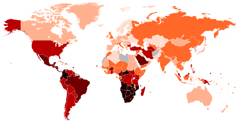
4. Concentration measures: Concentration measures study how the total values of a variable are distributed. The most important concentration measures are the Lorenz curve and the Gini index. They are used in multiple fields like the study of economic inequality.
In economics, the Lorenz curve is a graphical representation of the distribution of income or of wealth. It was developed by Max O. Lorenz in 1905 for representing inequality of the wealth distribution.
The curve is a graph showing the proportion of overall income or wealth assumed by the bottom x% of the people, although this is not rigorously true for a finite population (see below). It is often used to represent income distribution, where it shows for the bottom x% of households, what percentage (y%) of the total income they have. The percentage of households is plotted on the x-axis, the percentage of income on the y-axis. It can also be used to show distribution of assets. In such use, many economists consider it to be a measure of social inequality.

The Gini coefficient measures the inequality among values of a frequency distribution, such as the levels of income. A Gini coefficient of 0 expresses perfect equality, where all values are the same, while a Gini coefficient of 1 (or 100%) expresses maximal inequality among values. For example, if everyone has the same income, the Gini coefficient will be 0. In contrast, if for a large number of people only one person has all the income or consumption and all others have none, the Gini coefficient will be nearly one.
Atkinson index: The Atkinson index (also known as the Atkinson measure or Atkinson inequality measure) is a measure of income inequality developed by British economist Anthony Barnes Atkinson. The measure is useful in determining which end of the distribution contributed most to the observed inequality. The index can be turned into a normative measure by imposing a coefficient to weight incomes. Greater weight can be placed on changes in a given portion of the income distribution by choosing 
The Atkinson index is defined as:

where 

Entropy: The formula for general entropy for real values of 

where N is the number of cases (e.g., households or families),
Inequality measures based on quantiles: statistical measures based on quantiles are frequently applied to the analysis of income distribution as they comprise many popular inequality and poverty indices and indicators. Simple dispersion ratios, defined as the ratios of the income of the richest quantile over that of the poorest quantile, usually utilize deciles and quintiles, but in principle, any quantile of income distribution can be used. These measures do not depend on changes in scale and allow comparison of low, middle, and high income groups.
References: