Driver Profiling through ML

Project: https://github.com/octadelsueldo/TFM_Driver_Profiling

Authors:

Octavio del Sueldo 

Jose Lopez

Supervisor

Juan Manuel López Zafra

Abstract: Traffic accidents represent a high cost for insurance companies as well as for society, in economic and social terms, because in all cases the costs include medical and rehabilitation ex- penses, legal and emergency services, property damage and production losses. Thanks to the use of telematics and data science we may be able to find patterns of behavior that explain the claims. During this research we will work with a database of more than 95,000 drivers that includes infor- mation collected over 6 years; for this, we have performed an important work of cleaning and engi- neering of variables, for finally clustering the drivers through a PAM, being the most representative variables the intensity of use of the vehicle and the driving experience. In addition, we have made a prediction based on whether or not they have suffered a crash using a decision tree, obtaining a 72.25% accuracy rate.

“We highlight Intensity of use and experience as the most decisive variables when it comes to explaining crashes”

1. Introduction.

Insurance is an effective way of protecting individuals against the consequences of risks. It is based on transferring the risks to an insurer who is responsible for compensat- ing all or part of the damage caused by the occurrence of an event. A fair price will accu- rately reflect the actual risk of the insured, otherwise the business may have problems in the client portfolio, since those clients who have less risks end up supporting those who are riskier, which causes a client ́s churn with lower loss ratio and an entry of those with high loss ratio.... [1-4]

This directly harms insurance companies, policyholders and, consequently, society. Therefore, actuaries use risk-related information, i.e., they use those factors that model risk for insurance premium calculation, so that they can construct league tables based on expected losses.

In the case of automobiles, the traditional variables for determining the risk profile are personal characteristics, claims history and vehicle characteristics. However, premi- ums are often inaccurate in practice, as these factors do not have a direct causal relation- ship with actual driving risk.

Thanks to the development of networks, connectivity, IoT... UBI (Usage Based Insur- ance) products are increasingly popular within insurance companies. This insurance product model is based on schemes known as "pay-as-you-drive" (PAYD) and "pay-how- you-drive" (PHYD); the determination of the premium is based on variables determined from the actual data of the driver, such as driving time, distance traveled, type of roads traveled, speeds.... [5-7]

Thanks to the use of these technologies, the benefit is twofold, since the insured ob- tains a price that is more in line with his behavior, so that drivers with lower accident rates will not be penalized, and, on the other hand, insurance companies can effectively improve the accuracy of insurance prices. In addition, UBI products encourage drivers to drive less or improve their driving habits, as they can benefit from the use of dynamic premiums.

This coupled with the use of data science makes it possible to mine the information collected by the devices, so that insurers can fine-tune their risk models. Insurers can model driver behavior and therefore able to predict future claims based on what has hap- pened in the past.

According to studies on the subject, such as Ryan et al. (1998) [8-11], young drivers are those with the highest accident rates, which is why we will focus on this profile of drivers, specifically, drivers between 18 and 30 years of age.

As we have already mentioned, the main objective of our research is to segment young drivers based on their driving characteristics, driver information, such as age and vehicle qualities (power, weight, etc.). This segmentation (unsupervised algorithm) will help to classify drivers, using a decision tree (supervised algorithm), based on their acci- dent rate, for which we will use the proxy of crashes (decelerations of more than 4G).

2. Goals of the Project

• Database cleaning

• Identification of essential variables.

• Identification of groups of drivers and behavior patterns

• Prediction by classification tree.

• Proposal for a scorecard.

3. Analysis

3.1. Exploratory Data Analysis

First, we perform an exploratory analysis of the database in order to find possible data quality failures.

3.2. Feature Engineering

Once this phase is done, we start with the feature engineering. The first thing will be to perform an imputation of null values ​​(each variable was studied separately). We have also carried out a transformation of variables changing the units of measurement, for example from meters to kilometers. Likewise, we have deleted variables that we do not consider relevant for the analysis, either due to knowledge of the business or due to multicollinearity with other variables. In addition, we have created new variables that have been essential for the explanation of our unsupervised clustering model, such as the intensity of vehicle use. In this section we have also defined the target variable as a dummy variable that takes the value zero if there is no crash and the value one if there is a crash. Finally, given the objectives of the work, we have filtered our database, keeping only those young drivers between 18 and 30 years old, as well as those drivers who had a minimum of 60 registrations and 30 days in the product.

3.3. Relevant variables

In a later step, we have carried out an exploratory analysis of the data already filtered by the engineering phase with the aim of obtaining insights on the behavior of these drivers. Thanks to this, we were able to determine that the intensity of vehicle use is related to the number of crashes. Being those drivers with the highest intensity of use the ones that present the greatest crashes. In addition, the experience behind the wheel is another of the variables that explain the number of crashes, so that the less experienced drivers are the ones who present the greatest crashes. After these analyses, we have studied the gender variable and we can conclude that men have a higher accident rate than women.

3.4. Clustering

Once the most relevant variables have been determined, we have carried out a clustering through a PAM using the Euclidean distance. To do this, we have determined the optimal number of groups through the elbow rule, resulting in two as the optimal number of groups. Segmenting the dataset, we have obtained a silhouette of 0.25 and two groups that are well differentiated by their characteristics. The first of these corresponds to young drivers who have an average age of less than 25 years and experience behind the wheel of close to 5 years. These drivers use the vehicle more times a day, so they are more exposed to risks, which causes crashes in this group to be higher. On the other hand, the second cluster is made up of the most experienced drivers with an average age close to 29 years and an average experience of more than 9 years. In this case, drivers have fewer crashes due to the learning factor and use the vehicle less times per day, so they are less exposed to crashes.

3.5. Prediction using a decision tree

This is where we will take advantage of the groups of drivers and their qualities to predict whether or not they will crash. We have used a decision tree as it is one of the easiest models to interpret for people without technical knowledge of algorithms. Once our environment is initialized in PyCaret, we have defined the number of initial leaves with which we should work the decision tree in such a way that it allows us to obtain the highest Accuracy possible. Likewise, we have tuned our model so that it allows us to better classify those drivers that had crashes within our dataset since, as the classes were unbalanced, our model classified the zeros very well, but left aside the ones of our model, so what we did was assign different weights to each of the classifiers according to the needs of the business. This is where we have assigned a profit of EUR 4000 for those true positives, that is, those that we predict as crash and are effectively crash since if we can identify them we can charge a higher premium to these drivers. On the other hand, we will allocate a reward of EUR 2,500 for those drivers who are identified as not crashing and are effectively not crashing as we will reward them for their good driving, but at the same time we will save capital as they will not give us additional costs for have good driving habits. The false negatives will have a cost of EUR 3,000 since they would be drivers that we have identified as negative when they were positive, that is, we are going to charge them less and they will also crash, so they are the drivers we want to avoid. As for the false positives, we will put a cost of EUR 1000 on them since we will be charging them more than they should and they will also have no incidents driving so it is likely that they can find other alternatives on the market and go to the competition what we would lead to stop charging those premiums. Once this was done, we achieved superior results compared to our first model. We have decreased about 4 percentage points in Accuracy and also in Precision but we have improved the Recall and the F1 Score since now we are capturing more ones in our model and we go from a Recall of 0.02 to 0.219 while the F1 Score goes from 0.04 to 0.2738 . This leads us to the conclusion that by adding the costs to each of the classifiers according to the relative needs of the business we can outperform our base model.

4. Conclusions

After conducting exhaustive research on more than 95,000 drivers and 45 variables, from more than 54 million trips between 2007 and 2013, which determine driving behavior, vehicle characteristics and driver attributes, such as age , experience or sex, we can conclude that there are variables that explain the accident rate for drivers between 18 and 30 years old. Among these variables we highlight the experience behind the wheel or the intensity of use and the fact is that the greater the intensity of use, the greater the accident rate, this makes sense since the insured is more exposed to accidents, so by probability he should have a greater number of crashes, Experience is also decisive when it comes to explaining crashes, and the lesser the experience, the greater the number of crashes. In both cases, the relationship between sex was also studied, and men are always more prone to accidents than women. Thanks to the identification of these variables, we have carried out a segmentation of the conductors using a Partitioning Around Medoids (PAM). After studying the optimal number of groups, we determined that 2 is the one that maximizes the silhouette of the cluster using the elbow method. Using the Euclidean distance we obtain a mean silhouette of 0.25 and two groups of similar size:

• First group: They are younger and less qualified drivers; the average and maximum speed are slightly lower than those of the first group; however, the intensity of use is higher than average, almost 3 trips a day. Lastly, they have a higher than average accident rate

• Second group: These are the most experienced and older drivers, with higher average and maximum speeds; a possible explanation comes from the fact that they tend to drive on open roads with a higher intensity than in the urban cycle. The intensity of use (defined as the number of times the driver uses the car per day, as stated above) is slightly lower than that of the other group. Finally, the accident rate (measured in terms of collisions) is lower in this group than in the second.

Using the information provided by the unsupervised algorithm, we make a classificatory prediction of users who will or will not crash. For this, we use a decision tree, this is because it is one of the easiest models to interpret by people without technical knowledge. After optimizing the algorithm we have obtained the following metrics

• Accuracy: 72.25

• AUC: 61.64

• Recall: 21.9

• Accuracy: 36.40

• F1Score: 27.38

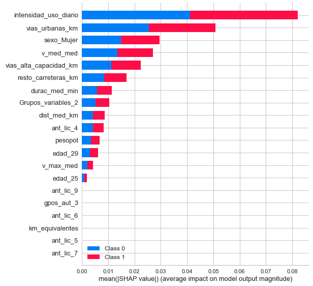
To achieve these results, we have assigned different weights to each of the possible classifiers in our algorithm, that is, the False Negative will not have the same weight as the True Positive, since they will be those that we treat as low-risk drivers, charging them a low premium when they will crash in the future. Beyond the results, one of the most important conclusions, which reinforces our initial hypotheses, is that the most significant variable for the tree is the intensity of vehicle use.

References

1. Zhang, H., Xu, L., Cheng, X., Chen, W., & Zhao, X. (2017). Big Data Research on Driving Behavior Model and Auto Insurance Pricing Factors Based on UBI. Lecture Notes in Electrical Engineering, 404–411. https://doi.org/10.1007/978-981-10-7521-6_49

2. Ma, Y. L., Zhu, X., Hu, X., & Chiu, Y. C. (2018). The use of context-sensitive insurance telematics data in auto insurance rate making. Transportation Research Part A: Policy and Practice, 113, 243–258. https://doi.org/10.1016/j.tra.2018.04.013

3. Sarabia, J. M., Prieto, F., Jordá, V., & Sperlich, S. (2020). A Note on Combining Machine Learning with Statistical Modeling for Financial Data Analysis. Risks, 8(2), 32. https://doi.org/10.3390/risks8020032

4. Guillen, M., & Pesantez-Narvaez, J. MACHINE LEARNING AND PREDICTIVE MODELING FOR AUTOMOBILE INSURANCE PRICING MACHINE LEARNING Y MODELIZACIÓN PREDICTIVA PARA LA TARIFICACIÓN EN EL SEGURO DE AUTOMÓVILES.

5. Huang, Y., & Meng, S. (2019). Automobile insurance classification ratemaking based on telematics driving data. Decision Support Systems, 127, 113156. https://doi.org/10.1016/j.dss.2019.113156

6. Bordoff, J., & Noel, P. (2010). Pay-as-you-drive auto insurance. Issues of the Day: 100 Commentaries on Climate, Energy, the Environment, Transportation, and Public Health Policy, 150.

7. Bolderdijk, J., Knockaert, J., Steg, E., & Verhoef, E. (2011). Effects of Pay-As-You-Drive vehicle insurance on young drivers’ speed choice: Results of a Dutch field experiment. Accident Analysis & Prevention, 43(3), 1181–1186. https://doi.org/10.1016/j.aap.2010.12.032

8. Ryan, G., Legge, M., & Rosman, D. (1998). Age related changes in drivers’ crash risk and crash type. Accident Analysis & Prevention, 30(3), 379–387. https://doi.org/10.1016/s0001-4575(97)00098-5

9. Lifestyle and accidents among young drivers. (1994, 1 junio). ScienceDirect. https://linkinghub.elsevier.com/retrieve/pii/0001457594900035

10. Machin, M. A., & Sankey, K. S. (2008). Relationships between young drivers’ personality characteristics, risk perceptions, and driving behaviour. Accident Analysis & Prevention, 40(2), 541–547. https://doi.org/10.1016/j.aap.2007.08.010

11. Tränkle, U., Gelau, C., & Metker, T. (1990). Risk perception and age-specific accidents of young drivers. Accident Analysis & Prevention, 22(2), 119–125. https://doi.org/10.1016/0001-4575(90)90063-q

12. Patil, P. (2018, July 7). What is Exploratory Data Analysis? — Towards Data Science. Medium. https://towardsdatascience.com/exploratory-data-analysis-8fc1cb20fd15

13. Reid Turner, C., Fuggetta, A., Lavazza, L., & Wolf, A. L. (1999b). A conceptual basis for feature engineering. Journal of Systems and Software, 49(1), 3–15. https://doi.org/10.1016/s0164-1212(99)00062-x

14. Rençberoğlu, E. (2019, 3 abril). Fundamental Techniques of Feature Engineering for Machine Learning. Medium. https://towardsdatascience.com/feature-engineering-for-machine-learning-3a5e293a5114

15. Kalsoom, R., & Halim, Z. (2013). Clustering the driving features based on data streams. INMIC. Published. https://doi.org/10.1109/inmic.2013.6731330

16. Higgs, B., & Abbas, M. (2013, October). A two-step segmentation algorithm for behavioral clustering of naturalistic driving styles. In 16th International IEEE Conference on Intelligent Transportation Systems (ITSC 2013) (pp. 857–862). IEEE.

17. Hanafy, M., & Ming, R. (2021). Machine learning approaches for auto insurance big data. Risks, 9(2), 42.

18. Silhouettes: A graphical aid to the interpretation and validation of cluster analysis. (1987, 1 november). ScienceDirect. https://www.sciencedirect.com/science/article/pii/0377042787901257

19. Model-based evaluation of clustering validation measures. (2007, 1 march). ScienceDirect. https://www.sciencedirect.com/science/article/abs/pii/S0031320306003104

20. Arora, P., Deepali, & Varshney, S. (2016, 1 January). Analysis of K-Means and K-Medoids Algorithm For Big Data. ScienceDirect, 78. https://www.sciencedirect.com/science/article/pii/S1877050916000971

21. Chakure, A. (2020, 6 November). Decision Tree Classification — The Startup. Medium. https://medium.com/swlh/decision-tree-classification-de64fc4d5aac

22. Moral-García, S., Castellano, J. G., Mantas, C. J., Montella, A., & Abellán, J. (2019). Decision tree ensemble method for analyzing traffic accidents of novice drivers in urban areas. Entropy, 21(4), 360.

23. Galarnyk, M. (2021, January). Understanding Decision Trees for Classification (Python). Medium. https://towardsdatascience.com/understanding-decision-trees-for-classification-python-9663d683c952

24. Rane, S. (2019, 9 November). SHAP: A reliable way to analyze model interpretability. Medium. https://towardsdatascience.com/shap-a-reliable-way-to-analyze-your-model-interpretability-874294d30af6

25. Dataman. (2021, 2 May). Explain Your Model with the SHAP Values — Towards Data Science. Medium. https://towardsdatascience.com/explain-your-model-with-the-shap-values-bc36aac4de3d